Module "Portfolio Service Extended Portfolio Analysis"
In the Infront Portfolio Manager, the following instruments can be viewed in detail as part of the individual or distribution analysis:
-
Shares
-
Fund
-
Accounts
-
Bonds (zero bonds, coupon bonds, floaters) for whose currency interest rate structures are available
-
Warrants (options) on bonds or shares
No individual or distribution analysis can be carried out for other instruments such as certificates and other derivative products. Here, however, it is possible to treat the entire portfolio (group, holder, custody account) as a fund and thus determine a VaR for the portfolio. Loans, fixed-term deposits and forward exchange transactions (if valuation rates have been entered) are also taken into account.
Risk models can be divided into two classes: Simulation models and parametric models. The Infront Portfolio Manager uses a parametric model, the so-called delta-normal model - also known as the variance-covariance method.
The price of an instrument V(t) is modeled as a (linear) function of the values (usually prices) Si (t ) of the risk factors (i=1...n) influencing the price: V(t):=(Δ1 S1 (t),...,Δn Sn (t)). Where Δi=∂V/(∂Si ), i.e. the change in the price of the instrument caused by the change in the price of the ith risk factor.
The logarithmic returns of the risk factors are assumed to be normally distributed.
The following market parameters (risk factors) are taken into account in the model for the above-mentioned instruments:
|
Security type |
Market parameters |
|---|---|
|
Shares |
Share price, Δ=1 |
|
Fund |
Fund price, Δ=1 |
|
Accounts |
- |
|
Bonds |
Discount factors of the (risk-free) yield curve (see excursus), Δ=1 |
|
Options |
Risk factors of the underlying instrument. In the model weighted with the option delta ( Δ ) in the Black-Scholes model |
If the evaluation currency and the currency in which the instrument is quoted are different, a risk resulting from a possible (negative) change in the exchange rate D(t) must also be taken into account. The exchange rate therefore also represents a risk factor.
However, due to certain model-related reasons, exchange rates are not treated as additional risk factors, but are taken into account using a special method (volatility transformation, see Deutsch, 31.3).
Excursus: Valuation of interest rate instruments
Interest rate instruments such as coupon bonds, zero bonds and floaters can be valued using the present value method: If interest payments Z(tj) are due at times T≥tj≥t during the remaining term of the bond between the valuation time t and the final maturity T , the bond is worth just the sum of the interest payments Z(tj) discounted with the discount factors B(t,tj) at time t :
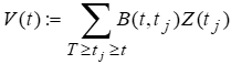
In the case of coupon bonds and zero bonds, the expected future interest payments are known. For floaters where the interest rate is variable for the future, an interest payment for the valuation can be obtained from arbitrage considerations.
The discount factors result from the current interest rate situation (and the credit rating) of the bond issuer.
For bonds, the cash flow decomposition described in the excursus is carried out to determine the associated discount factors as risk factors.
Excursus: Yield curves in the Infront Portfolio Manager
Yield curves are derived from the structure (interest rate, interest day method, interest dates, term, etc.), prices and other market data of bonds traded on the market. Market data are, for example, YTM (yield-to-maturity), swap rates, par rates, money market rates, etc. Assuming no arbitrage, a discount factor B(t,T) for discounting a payment due at time T to time t can be determined from these various market data (assuming the same credit rating). Bootstrapping is used to obtain the discount factors (or the underlying spot rate curve).
In the Infront Portfolio Manager, the interest rate structure is obtained by bootstrapping from the Tullett swap curve stored in the yield curve configuration. Money market rates are used as input for residual terms of up to one year and benchmark swap rates for longer residual terms.
The (base) interest rate structure obtained in this way applies to quasi risk-free bonds (such as German government bonds). For individual bonds, whose issuer default risk is generally higher, a spread on the basic interest rate structure is calculated from their market prices, which is constant for all supporting points, resulting in the creditworthiness-dependent interest rate structure as the basic interest rate structure + spread.
As only time series at certain grid points (for which the swap or money market data are available) are available for the yield curves, a risk-based cash flow mapping must still be carried out.
Excursus: Risk-based cash flow mapping
The actual interest payments at any points in time ∞>tj≥0 are transformed into interest payments at the sampling points tk,k=1...l . Important here is the term risk-based, which means that both the present value and the risk are invariant with regard to this transformation (cf. Deutsch, 24.2.2),
The value at risk for a risk factor for
-
a forecast period of δt periods
-
with given probability w
now results in
VaR:=|ΔN-1 (w)σ√δt|
The value at risk for a risk factor for
σ here denotes the standard deviation of the logarithmized period returns, N-1 (w) the inverse cumulative normal distribution.
For a portfolio with several risk factors (due to different instruments or due to the discount factor modeling of the bonds), it is assumed that these are interdependent. The dependency is modeled in the form of a correlation.
In the case of m risk factors, the value at risk is ultimately calculated as
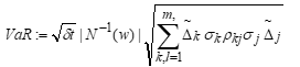
σk denotes the standard deviation of the kth risk factor, ρkj the correlation between the risk factors k and I.
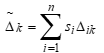
where si denotes the portfolio of instrument i (n instruments, i=1...n) and Δik stands for the delta of instrument i with respect to the risk factor k. If the risk factor k has no influence on the price of the instrument i, then Δik:=0.
Both the standard deviation and the correlations are EMWA estimates (i.e. not the historical mean values found elsewhere in the program). If necessary, read German, 32.