Basic key figures

Basic key figures as time series

The following key figures are available as time series. (MM-Talk return value: Time series)

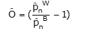
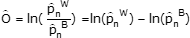
Outperformance

Outperformance is defined as the (percentage) increase or decrease in income over a period of n periods (i.e. depending on the consolidation):

	on the basis of absolute performance
	on the basis of the logarithmized return

MM-Talk: TimeSeries.Outperformance[$BasicTimeSeries;$Periods;$logReturns]

The annualized outperformance is shown in the analysis.

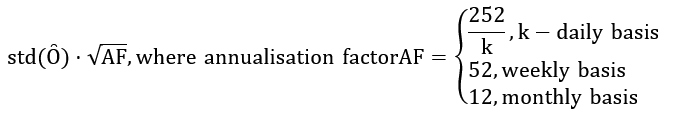
Stability of outperformance

The stability of the outperformance is defined as the annualized standard deviation(std) over n sample periods (see preliminary remark) of the outperformance time series in a period of n periods (i.e. depending on the consolidation):

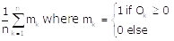
Probability of outperformance

The probability of outperformance is defined as the quotient of the number of periods with positive outperformance and the number of observation periods n in a period of n periods (i.e. depending on the consolidation):

Tracking error

The tracking error is defined as the annualized standard deviation over n sample periods of the difference time series of security performance and underlying security performance (see preliminary remarks).

For the logarithmic returns, it is formally equal to the stability of the outperformance:

Basic key figures as individual key figures for an evaluation date

All of the following key figures are available as individual key figures for an evaluation date. (MM-Talk return value: Number)

The following key figures are the result of a regression analysis. The aim here is to show the return on a security as a function of the return on a benchmark:

^ȓW=F(^ȓB)+ε

The aim is to minimize the error ε.

Depending on the parameters of the MM-Talk functions, the absolute return ȓ'=p̑-1or the logarithmized return is used.

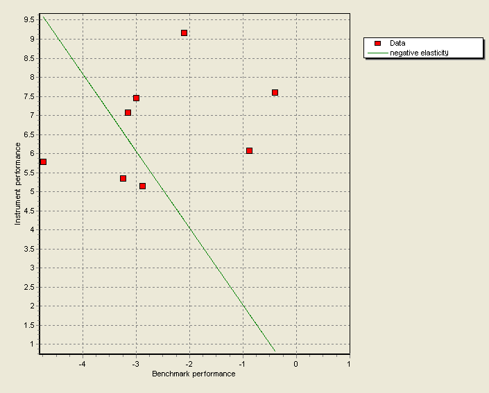
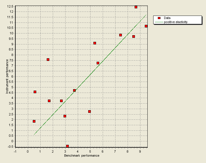
The calculation of the positive and negative elasticities is based on the model that, on the one hand, rising and falling market phases are to be observed separately and thus also examined, and on the other hand, no management performance (for funds) can be determined. This results in a linear regression model that is calculated with data over n periods.

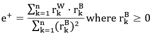
Positive elasticity

For the positive elasticity, i.e. the dependence of security performance in a rising market phase on the underlying security performance, the model is

^ȓW=e+⋅ȓB

with the optimal solution

MM-Talk: TimeSeries.PositiveReturnElasticity[$BaselineTimeSeries;$Periods;
$EvaluationDate;$logReturns]

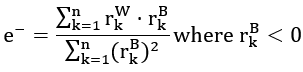
Negative elasticity

For negative elasticity, i.e. the dependency of security performance in a falling market phase on the underlying security performance, the model is

^ȓW=e-⋅ȓB

with the optimal solution

MM-Talk: TimeSeries.NegativeReturnElasticity[$BaselineTimeSeries;$Periods;
$EvaluationDate;$logReturns]