Residual terms of the multi-period attribution

Module "Portfolio Service Extended Portfolio Analysis"

Two different types of residual terms occur in the performance attribution (B): Temporal residuals resulting from the geometric combination of several periods and interaction terms when calculated in relation to a benchmark (sometimes called "cross product" or simply "residual").

Temporal residuals (time residuals, temporal coupling terms)

These inevitably occur if an attribution is carried out with more than one segment over several periods. It is irrelevant whether the segments are "real" portfolio segments such as "equities", "bonds" or "fixed-term deposits" or hypothetical segments such as "allocation contribution", "selection contribution" or "residual contribution".

Let's look at an example with two periods and two segments. We decompose the performance of the portfolio in the first period as

_{P1=α1A1+β1B1}

where_A1 is the performance of the first segment and α1 is_the weight of the first segment at the beginning of the period and_B1 is the performance of the second segment and_β1 is the weight of the second segment at the beginning of the first period. Similarly, we write with analogous designations for the second period

_{P2=α2A2+β2B2}

The performance of the portfolio over both periods is as follows

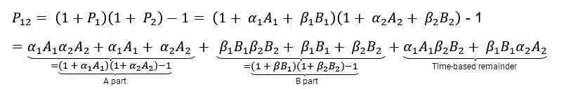
The A component is therefore just the sum of the terms that only contain contributions belonging to A (_A1,_A2,_α1,_α2). Similarly, the B component is the sum of the terms that only contain variables belonging to B.

It is noticeable that the A (B) share is precisely the geometric combination of the performance contributions of segment A (B) over the two periods.

The temporal remainder now consists of the terms that do not clearly belong to either A or B. This means that the sum of the performance contributions over several periods is only equal to the total performance if the temporal remainder is 0 (which almost never occurs).

The time residual is shown in the performance attribution evaluation with benchmark as a "time residual". The "time residual (contributions)" is the residual obtained by entering "Allocation", "Selection" and "Residual" as segments in the above calculation. The variable "time residual (surplus)" is obtained by setting the performance of the portfolio segment for A, the weight of the portfolio segment for α, the weight of the corresponding benchmark segment for β and the performance of the corresponding benchmark segment for B in the above calculation. Then the excess performance of a period is _{ΔP1=α1A-β1B} and we obtain the temporal remainder of the excess performance exactly as above (but of course with a negative sign).

Example

Let's look at a portfolio consisting of a share portfolio and an overnight money account. The following transactions are given:

In the first period from 1.2.08 (after purchase) to 1.8.08 (before sale), the performance of the securities account was 400/440-1 = -9.09%. The performance of the account segment in the first period is 578/560-1=3.21%.-1=3.21%.

In the second period from 1.8.08 (after sale) to 31.12.08, the portfolio performance was 140/200-1=-30% and the account performance 794/778-1=2.06%.

This results in a performance contribution of the portfolio for the first period of_PD1=44%*(-9.09%)=-4% and in the second period of_PD2=20%*(-30%)=-6%.

Similarly, this results in a performance contribution for the account of_PK1=56%*3.21%=1.8% in the first period and_PK2=80%*2.06%=1.65% in the second period.

If we now add up the performance contributions for the account and securities account over both periods, we obtain the following using a geometric linkage

_PK=(_1+PK1 )(_1+PK2 )-1 = 1.018 * 1.0165 -1 = 3.48%

and

_PD=(_1+PD1 )(_1+PD2 )-1 =0.96*0.94-1= -9.8%

If we now calculate the performance of the entire portfolio, we get

_PP=(_1+PK1+PD1 )(_1+PK2+PD2 )-1=(1+0.018-0.04)*(1+0.0165-0.06)-1=-6.45%

This means that the temporal remainder in this case is_PP-PK-PD=-0.13%.